Build and Edit a MOM6 Grid in Jupyter
This tutorial works through the following operational elements using the grid generation application and library functions:
Prerequisites
This tutorial assumes the gridtools software has been installed. A local installation tutorial is available.
It is also assumes that a jupyter lab session is also available.
This tutorial does not cover any details on the controls in the grid generation application. Please see “Grid Generation” for details on the controls in the application.
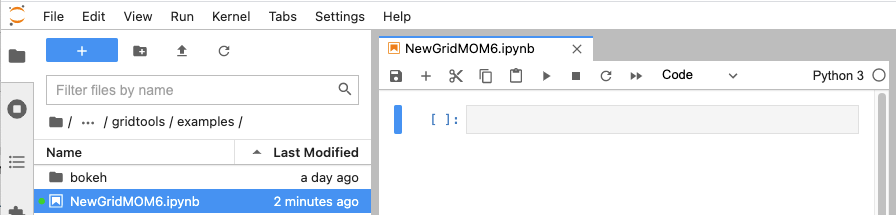
An existing notebook with the complete code can be found in the
examples
directory of the github repository. The name of the example
is NewGridMOM6.ipynb.
This tutorial assumes that code is being systematically added
cell by cell. Subsequent sections of code need to be set to
True to allow those code blocks to run.
The GEBCO 2020 topographic dataset is needed for this example.
Be sure the GEBCO_2020.nc is available for use. The source
of this dataset is
available here.
This example will run on the binder website. Please follow these
“instructions” to
download the GEBCO_2020.nc dataset for use with binder.
Build an initial grid
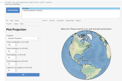
The first step is to load the gridtools library. The second step is creating a gridtools object and then launching the grid generation application.
Starting the grid generation application
Create three notebook cells. Each cell will have its own blocks of code. When each cell is run, a number will appear in the brackets. It is not important that the numbers match between your notebook and the tutorial.
[1]:
# Load some basic python libraries
import os, cartopy
# This loads the GridUtils portion of the gridtools library
from gridtools.gridutils import GridUtils
[2]:
# Create a GridUtils object
grd = GridUtils()

# Create a grid generation application object
grdGenApp = grd.app()
[3]:
# Launch the grid generation application within Jupyter
display(grdGenApp)
While working with the application, all grid information is stored
internally with the grd python object created above in cell #2.
Once work is completed with the application, the grd object will
be used to plot and further manipulate the model grid.
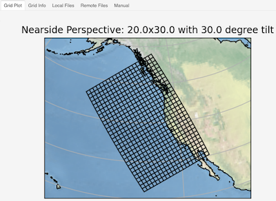
Using the default start up settings of the grid generation application will generate a 20x30 ocean model grid in the Lambert Conformal Conic projection centered at 40 degrees North and 230 degrees West.
For additional details about the operation of the grid generator, such as adjusting plot, grid parameters and other parameters, please see “Grid Generation”.
Please click on “Grid” next to the “Plot” tab. In the “Center”, tab, please click on “Make Grid”.
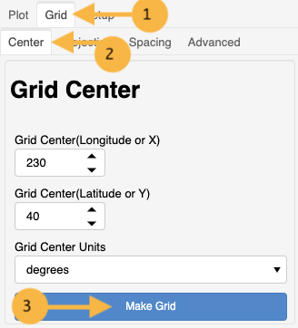
The area below “Grid Plot” should update and display a 20x30 ocean model grid.
The new grid is stored with the grd object and can be
used to generate roughness and topography grids.
Obtain roughness and topography grids
The location of the GEBCO 2020 file needs to be set appropriately.
[4]:
# Detach logger from application
grd.detachLoggingFromApplication()

# Source of GEBCO 2020 topographic grid
highResTopographyFile = "/import/AKWATERS/jrcermakiii/bathy/gebco/GEBCO_2020.nc"

if os.path.isfile(highResTopographyFile):
    topoGrids = grd.computeBathymetricRoughness(highResTopographyFile,
        depthName='elevation',
        maxMb=99, superGrid=False, useClipping=False,
        auxVariables=['depth'])
The routine computeBathymetricRoughness is called with the location of
the GEBCO 2020 topography. This routine normally only returns a
roughness calculation (h2). As seen above, a request was made for
the depth grid. Since GEBCO 2020 topographic grid is an
elevation we have to turn the depth grid into a
depth by taking the negative of the grid.
[5]:
# Turn the diagnosed topography grid into an actual depth
topoGrids['depth'] = -(topoGrids['depth'])
Write FMS coupler and mosaic files
Let us write the FMS coupler and mosaic files for the current model
grid, roughness and topography. Edit the wrkDir variable so
it points to an empty directory. A subdirectory called INPUT will
also need to be created.
In a later step, the model grid is rewritten. This can be to
the existing INPUT directory or another directory INPUT2
to allow comparison.
[6]:
# Write current model grid files
wrkDir = "/home/cermak/workdir/configs/zOutput"
inputDir = os.path.join(wrkDir, "INPUT")
input2Dir = os.path.join(wrkDir, "INPUT2")

# Write FMS coupler and mosaic files
grd.makeSoloMosaic(
    topographyGrid=topoGrids['depth'],
    writeLandmask=True,
    writeOceanmask=True,
    inputDirectory=inputDir,
    overwrite=True
)

# Write topographic variable
topoGrids.to_netcdf(os.path.join(inputDir, 'ocean_topog.nc'),
        encoding=grd.removeFillValueAttributes(data=topoGrids))

# Write the model grid
grd.saveGrid(filename=os.path.join(inputDir, "ocean_hgrid.nc"))
Note
By default, makeSoloMosaic will only output the files
needed by the FMS coupler. Two extra parameters were provided
to write an ocean and land mask. These will be used
later for the ocean mask editor. The land and ocean masks
are impacted if additional parameters, MASKING_DEPTH or
MINIMUM_DEPTH, are specified. If these are not specified,
these default to a depth of zero (0.0) meters. For more
details, see makeSoloMosaic().
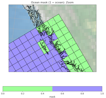
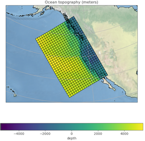
Examine the topography grid
In this section, two graphics are prepared. The first is a look at the current topography grid. The second graphic is the ocean mask.
Let us take a closer look at the model grid by plotting a high resolution coastline over the topography.
First, some plot parameters have to be specified. The
function plotGrid() is
called. This function returns figure and axes matplotlib objects
that can be further manipulated. The figures are displayed
by using a display() function.
[7]:
# Examine the topography grid
grd.setPlotParameters({
    'figsize': (8,8),
    'projection': {
        'name': 'LambertConformalConic',
        'lon_0': 230.0,
        'lat_1': 25.0,
        'lat_2': 55.0
    },
    'extent': [-160.0 ,-100.0, 20.0, 60.0],
    'iLinewidth': 1.0,
    'jLinewidth': 1.0,
    'showGridCells': True,
    'iColor': 'k',
    'jColor': 'k',
    'transform': cartopy.crs.PlateCarree(),
    'satelliteHeight': 35785831.0
})
(figure, axes) = grd.plotGrid(showModelGrid = True,
        plotVariables={
        'depth': {
            'values': topoGrids['depth'],
            'title': 'Ocean topography (meters)',
            'cbar_kwargs': {
                'orientation': 'horizontal',
            }
        }
    })
display(figure)

# Examine the ocean mask
oceanMask = grd.openDataset(os.path.join(inputDir, 'ocean_mask.nc'))

# Define our own color map (same used in mask editor)
import matplotlib.pyplot as plt
land_color = (0.6, 1.0, 0.6)
sea_color  = (0.6, 0.6, 1.0)
maskCM = plt.matplotlib.colors.ListedColormap(
    [land_color, sea_color], name='land/sea')

# MOM6 places lon and lat in x and y
# x and y need to be lon and lat coordinates for the mask editor
oceanMask = oceanMask.rename({
    'x': 'lon',
    'y': 'lat'
})
oceanMask = oceanMask.set_coords(['lon', 'lat'])

(figureMask, axesMask) = grd.plotGrid(showModelGrid = True,
        plotVariables={
        'mask': {
            'values': oceanMask['mask'],
            'title': 'Ocean mask (1 = ocean)',
            'cmap': 'land/sea',
            'cbar_kwargs': {
                'orientation': 'horizontal',
            }
        }
    })
display(figureMask)

# Zoom in to take a closer look
grd.setPlotParameters({
    'extent': [-140.0 ,-120.0, 49.0, 59.0]
})

(figureMaskZoom, axesMaskZoom) = grd.plotGrid(showModelGrid = True,
        plotVariables={
        'mask': {
            'values': oceanMask['mask'],
            'title': 'Ocean mask (1 = ocean): Zoom',
            'cmap': 'land/sea',
            'cbar_kwargs': {
                'orientation': 'horizontal',
            }
        }
    })
display(figureMaskZoom)
When this cell is run, three plots should appear.
Ocean Topography
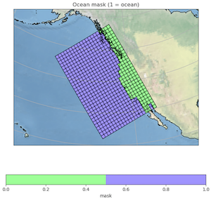
Ocean Mask Full Grid
Ocean Mask Zoomed
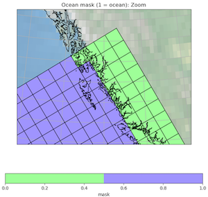
The ocean mask looks pretty good. In the next section, start the grid editor to change some of the points from ocean to land and land to ocean.
Use the editor to make some mask updates
To start up the mask editor, create a mask editor object with the desired projection. Create the mask editor application object and then use the display() function to launch the application.
For additional details about the operation of the grid editor, please see “Jupyter Mask Editor”.
[8]:
# Load the mask editor application module from gridtools
from gridtools.app import maskEditor

# Set a map projection for the mask editor to use
crs = cartopy.crs.Orthographic(-140, 45)

# Create the mask editor object
appObj = maskEditor(crs=crs, ds=oceanMask['mask'])

# Create the mask editor application object
app = appObj.createMaskEditorApp()

# Launch the application
display(app)
A successful launch of the application should look similar to the figure below. Start by selecting the zoom control and zooming into the same area as the figure above.
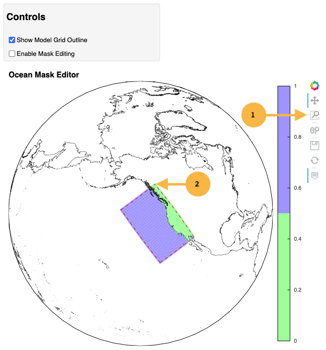
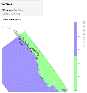
Once the zoom tool is selected, click and draw a box over the region to zoom. Releasing the mouse button should result in a redrawn map.
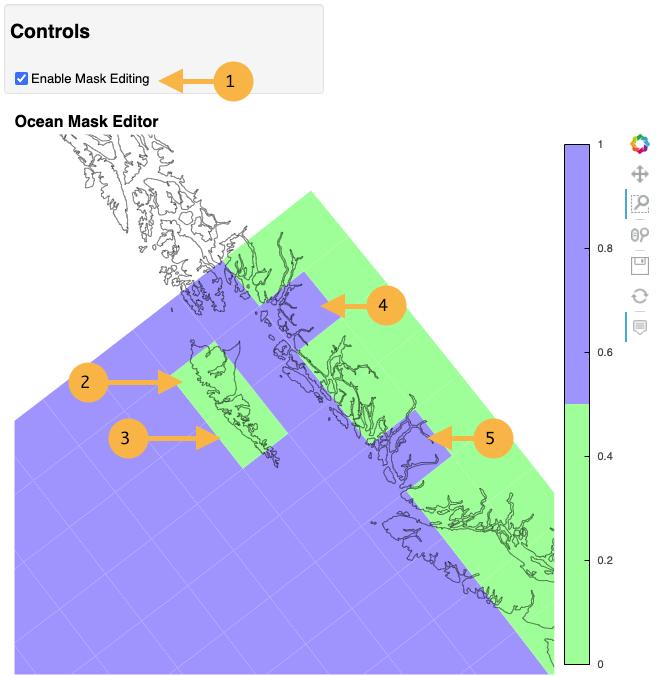
Clicking on the “Enable Mask Editing” checkbox, will allow mouse clicks on the grid to flip between land and ocean. Click two ocean boxes to change them to land. Click two land points to turn them to ocean.
The new ocean mask can be saved using the following code.
[9]:
# Save the new ocean mask
newMask = oceanMask['mask'].copy()
newMask = newMask.reset_coords(names = ['lat', 'lon'])
grd.saveDataset(os.path.join(inputDir, 'ocean_mask_new.nc'), newMask,
                overwrite=True, mapVariables = {'lon': 'x', 'lat': 'y'},
                hashVariables = ['mask', 'x', 'y'])
Apply mask changes to the model grid
The new ocean mask is applied to the current model grid. In this example, the default values are passed to MASKING_DEPTH, MINIMUM_DEPTH and MAXIMUM_DEPTH to show that these parameters can be set. Be sure that these match the parameter values specified in your MOM6 input files.
[10]:
# Apply new ocean mask to ocean model grid
topoGrids['depth'] = grd.applyExistingOceanmask(topoGrids, 'depth',
    os.path.join(inputDir, 'ocean_mask_new.nc'), 'mask',
    MASKING_DEPTH=0.0, MINIMUM_DEPTH=0.0, MAXIMUM_DEPTH=-99999.0)
Of the four points that were changed, this should be the expected result after running the above routine:
The (diagnosed) maximum depth of the ocean is 5413.075256 meters.
Beginning application of new ocean mask (changes noted, if any).
 * Number of land mask points with new depth of 0.000000: 2
 * Number of ocean points with new depth of 0.000000: 2
Warning
The two ocean points with a depth of 0.000000 in this case is incorrect. For MOM6, a MASKING_DEPTH set to 0.000000 means that depths of 0.000000 or shallower will be masked as land. When the MASKING_DEPTH and MINIMUM_DEPTH are EQUAL, an additional depth of epsilon is applied so the new point is actually an ocean point. The value of epsilon may need to be changed if the new ocean points are masked by MOM6.
See: applyExistingOceanmask() or
applyExistingLandmask() for
additional details.
Write updated FMS coupler and mosaic files
To finish the process of updating the model grid, the FMS coupler, mosaic, topography and model grid are written.
[11]:
# Rewrite FMS coupler and mosaic files
grd.makeSoloMosaic(
    topographyGrid=topoGrids['depth'],
    writeLandmask=True,
    writeOceanmask=True,
    inputDirectory=input2Dir,
    overwrite=True,
    MASKING_DEPTH=0.0, MINIMUM_DEPTH=0.0, MAXIMUM_DEPTH=-99999.0
)

# Be sure to save previously diagnosed `h2` grid
topoGrids.to_netcdf(os.path.join(input2Dir, 'ocean_topog.nc'),
        encoding=grd.removeFillValueAttributes(data=topoGrids))

grd.saveGrid(filename=os.path.join(input2Dir, "ocean_hgrid.nc"))
Check final ocean mask
Plot the final ocean mask to be sure the points are correctly represented.
[12]:
(figureMaskZoom2, axesMaskZoom2) = grd.plotGrid(showModelGrid = True,
        plotVariables={
        'mask': {
            'values': oceanMask['mask'],
            'title': 'Ocean mask (1 = ocean): Zoom',
            'cmap': maskCM,
            'cbar_kwargs': {
                'orientation': 'horizontal',
            }
        }
    })
display(figureMaskZoom2)